|
|
[Analyze]-[Convert Data]
[special]-[Fourier trans.]
This item is used to calculate Fourier transform of y(x). Please consult textbooks of mathematics about Fourier transform, and those of digital-signal analysis about DFT and FFT.
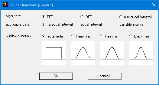
[algorithm] section
[FFT]
FFT (Fast Fourier transform) on the basis of Cooley–Tukey algorithm is used by selecting this option. This is applicable to a series of periodic data of 2N points with an equal interval, where N is an integer between 4 and 19.
[DFT]
DFT (discrete Fourier transform) is used by selecting this option. This is applicable to a series of periodic data with an equal interval. When you use FFT, the number of data must be 2N = 4, 8, 16, 32, 64, 128, 256, 512, 1024 and so on. In case of DFT, you can use the data numbers other than these. It will take much longer time to complete the calculation in DFT than FFT when the data number is large. But you don't realize the difference as long as the data number is small.
[numerical integral]
You can use this option for the data with variable interval and, of course, with equal interval. Even when a series of discrete data are obtained in experiments, their intervals are not always constant. Then you manage to make a equal-interval data from the raw data by, for example, a curve fit to utilize FFT or DFT. But you don't have to do so by using the present option. The calculation just follows the definition of Fourier transform; The numerical integral is carried out to get each Fourier coefficient. This means 100 integrals are needed to convert 100 points of y(x) to the Fourier coefficients. Thus it will take much longer time than FFT and even DFT. Even so, you will not realize the difference among FFT, DFT and the numericl integral when the data number is small — say 1000 or so — because of the amazing speed of today's PC.
[window function] section
It is known that artificial Fourier components sometimes appear due to the limitted number/lenngth of y(x). This is called side-lobe effect. A window function is multiplied to y(x) to suppress it. Three window functions are available in yoshinoGRAPH other than the "rectangular" one.
[rectangular]
This "function" is just a constant 1. Thus it does not do anything. The frequency resolution is the highest of the window functions.
[Hamming]
Hamming window is defined as below.
w(x) = 0.54 − 0.46 cos (2πx)
The frequency resolution of Hamming window is worse than the rectangular window, but better than Hanning window. The side-lobe effect is suppressed to an extent.
[Hanning]
Hanning window is defined as below.
w(x) = 0.5 − 0.5 cos (2πx)
The frequency resolution of Hanning window is worse than Hamming window, but the side-lobe effect is better suppressed.
[Blackman]
Blackman window is defined as below.
w(x) = 0.42 − 0.5 cos (2πx) + 0.08 cos (4πx)
The frequency resolution of Blackman window is the worst of the present window functions, but the suppression of the side-lobe effect is strongest.
|
